The Method

The goal of this post is to succinctly explain the main concepts used in the sample size computation method that powerly is based on. In doing so, I aim to help get you acquainted with terminology used throughout the rest of the posts in the tutorial section. You may regard this post as a summary of the key things discussed in Constantin et al. (2021).

Input

To start the search for the optimal sample size, powerly requires three inputs, namely, a true model, a performance measure, and a statistic.

True Model

The true model represents the set of hypothesized parameter values (i.e., the effect size) used to generate data during the first step of the method. These true parameter values are collected in a model matrix denoted $\mathbf{\Theta }$. One may either manually specify $\mathbf{\Theta }$ or generate it according to some hyperparameters via the generate_model function. The meaning and function of $\mathbf{\Theta }$ changes depending on context in which it is used. For example, in the context of psychological networks, $\mathbf{\Theta }$ encodes the edge weights matrix, where the ${\theta }_{ij}$ entries may represent partial correlation coefficients. However, in the Structural Equation Modeling (SEM), for example, $\mathbf{\Theta }$ may encode the model implied covariance matrix.

Performance Measure

The performance measure can be regraded as a quality of the estimation procedure relevant for the research question at hand. It takes the form of a function $f\left(\mathbf{\Theta },\hat{\mathbf{\Theta }}\right)$, where the $\mathbf{\Theta }$ argument is the matrix of true model parameters and $\hat{\mathbf{\Theta }}$ is the matrix of estimated model parameters. In essence, the performance measure is a scalar value computed by comparing the two sets of model parameters in $\mathbf{\Theta }$ and $\hat{\mathbf{\Theta }}$. Together with the performance measure, the researcher also needs to specify a target value $\delta$ indicating the desired value for the performance measure. Therefore, what constitutes an optimal sample size largely depends on what performance measure the researcher is interested in, which, in turn, is driven by the research question at hand.

Statistic

The statistic is conceptualized as a definition for power that captures how the target value $\delta$ for the performance measure should be reached. It takes the form of a function $g(\mathbf{\xi })$, where the argument $\mathbf{\xi }$ is vector of performance measures of size $R$ indexed by $r(r=1,...,R)$, with each element representing a replicated performance measure computed for a particular sample size.

Most commonly, this statistic may be defined in terms of the probability of observing a target value $\delta$ for the performance measure (i.e., analogous to a power computation) as:

$$\begin{array}{c}g\left(\mathbf{\xi }\right)=\frac{1}{R}\sum _{r=1}^R\left[{\xi }_r\ge \delta \right],\end{array}$$

where the notation $\left[\cdot \right]$ represents the Iverson brackets (Knuth, 1992), with $\left[{\xi }_r\ge \delta \right]$ defined to be $1$ if the statement ${\xi }_r\ge \delta$ is true and $0$ otherwise. Therefore, the optimal sample size needs to satisfy $g\left(\mathbf{\xi }\right)\ge \tau$, where $\tau$ is an arbitrary threshold indicating a certain probability of interest, i.e., the target value for the statistic.

Question

Taken together, the true model matrix $\mathbf{\Theta }$, the performance measure $f\left(\mathbf{\Theta },\hat{\mathbf{\Theta }}\right)$ with its corresponding target value $\delta$, and the statistic $g(\mathbf{\xi })$ with its target value $\tau$ allow one to formulate the following question:

Given the hypothesized parameters in $\mathbf{\Theta }$, what sample size does one need to observe $f\left(\mathbf{\Theta },\hat{\mathbf{\Theta }}\right)\ge \delta$ with probability $\tau$ as defined by $g(\mathbf{\xi })$?

powerly strives for flexibility, allowing researchers to provide custom implementations for performance measures and statistics that best suit their study goals. However, it also provides out of the box support for several models and common related performance measures. Check out the Reference Section for the powerly function for an overview of the currently supported models and performance measures.

TIP

Coming in powerly version 2.0.0 we are introducing an API that allows researchers to build upon and easily extend the current method to new models and performance measures. Check out the Developer Section for updates on the API design and examples on how to extend powerly.

Steps

Given the inputs presented above, the search for the optimal sample size is conducted in three steps, i.e., a Monte Carlo (MC) simulation step for computing the performance measure and statistic at various sample sizes, a curve-fitting step for interpolating the statistic, and a bootstrapping step to quantify the uncertainty around the fitted curve.

Step 1

The goal of the first step is to get a rough understanding of how the performance measure $f\left(\mathbf{\Theta },\hat{\mathbf{\Theta }}\right)$ changes as a function of sample size.

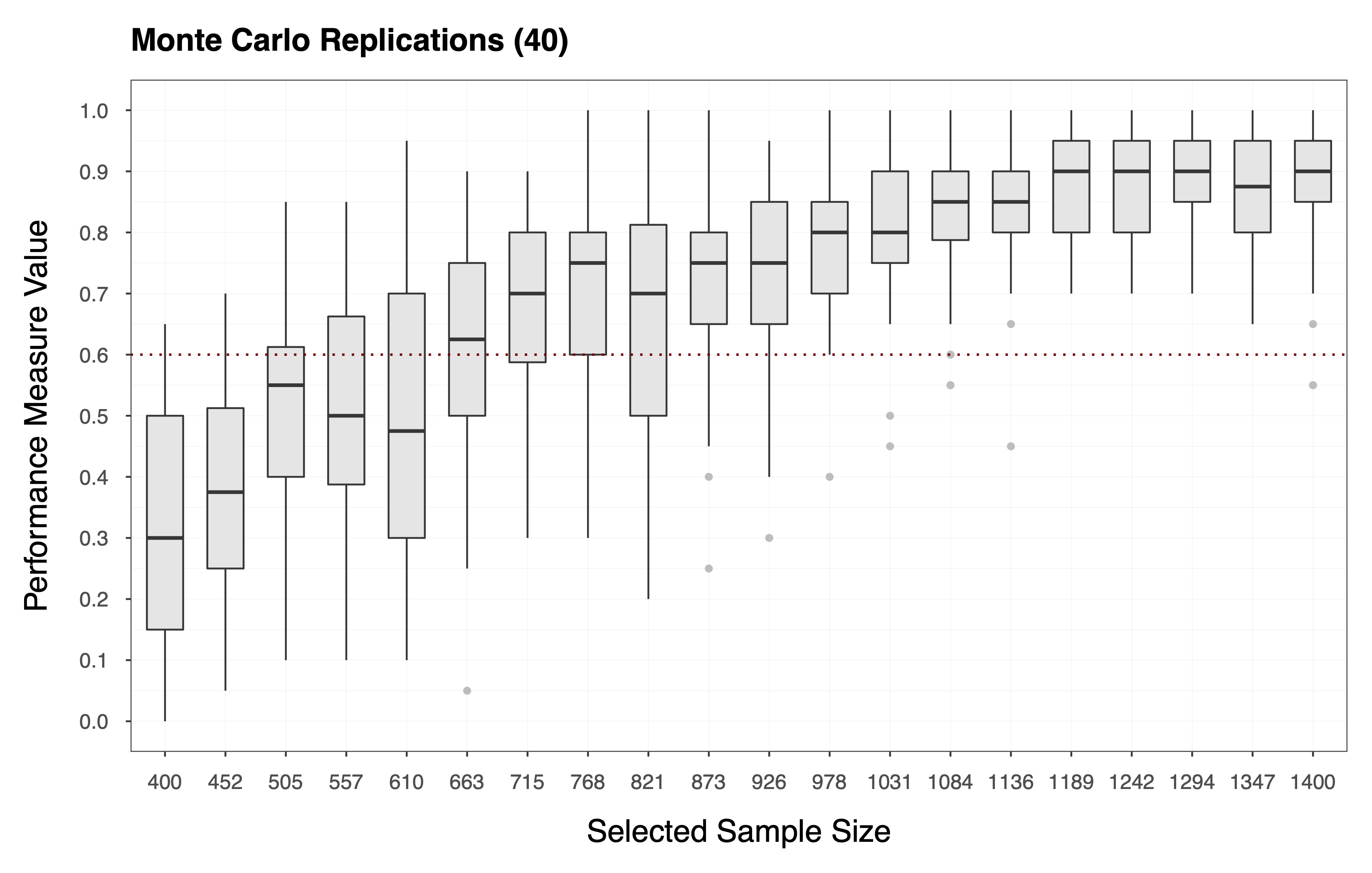
To achieve this we perform several MC simulations for different sample sizes selected from a candidate sample size range denoted ${\mathbb{N}}_s$, for example, ${\mathbb{N}}_s=[\mathrm{400..1400}]$. More specifically, we select $T$ indexed by $t(t=1,\dots ,T)$ equidistant samples as $S=\{s_1,\dots ,s_T\}\subseteq {\mathbb{N}}_s$. Then, for each $s_t\in S$, we perform $R$ MC replications as follows:

1. Generate data with $s_t$ number of observations using the true model parameters in $\mathbf{\Theta }$.
2. Estimate the model parameters matrix ${\hat{\mathbf{\Theta }}}^{(rt)}$ using the generated data.
3. Compute the performance measure by applying function $f\left(\mathbf{\Theta },{\hat{\mathbf{\Theta }}}^{(rt)}\right)$.

This procedure gives us an $R\times T$ matrix $\mathbf{\Xi }$, where each ${\xi }_{rt}$ entry is a performance measure computed for the $t$-th sample size, during the $r$-th MC replication. Each column of the $\mathbf{\Xi }$ matrix is, therefore, a vector ${\mathbf{\xi }}_t$ that holds the replicated performance measures associated with the $t$-th sample size (i.e., see the plot below).

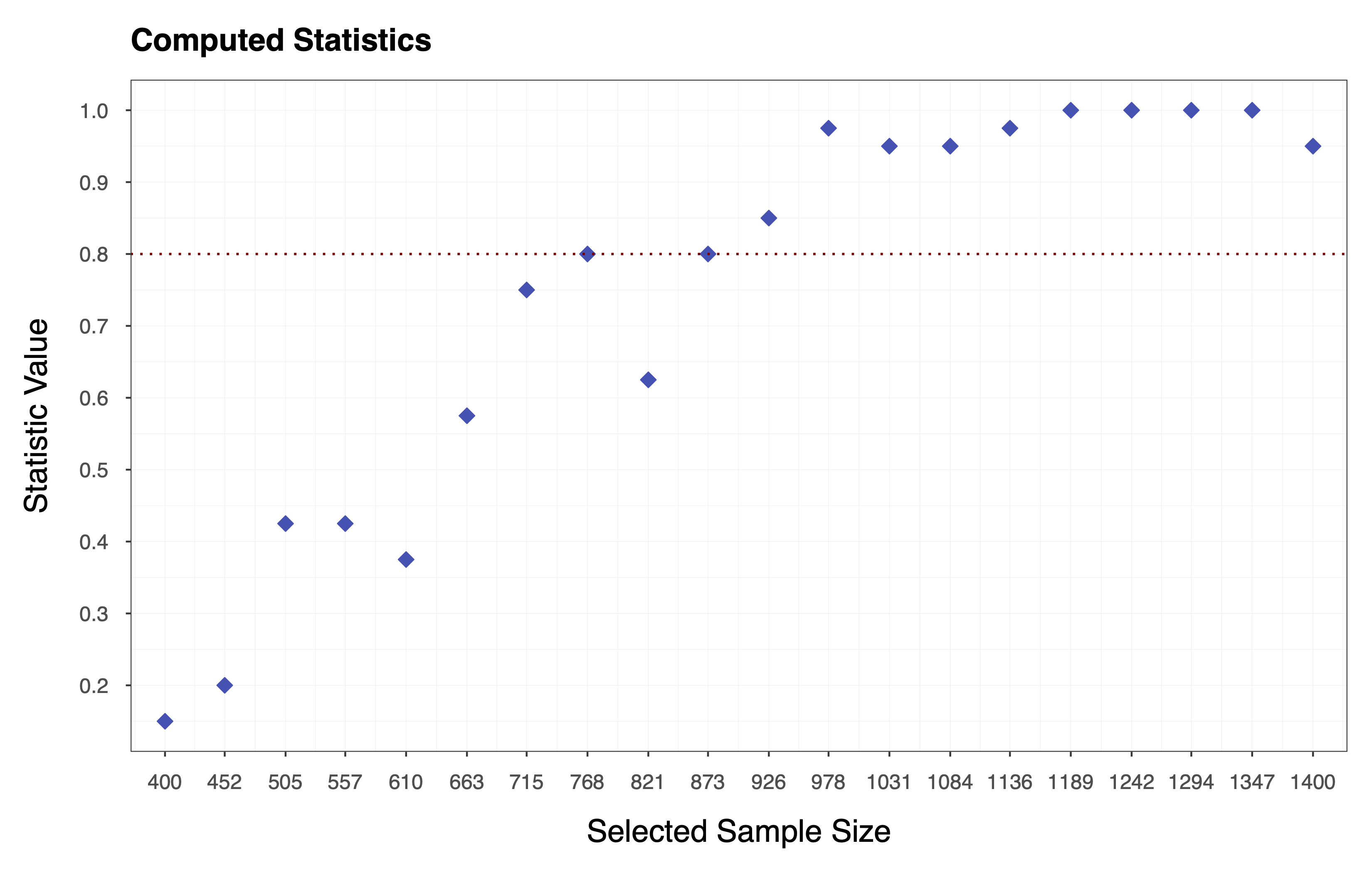
Finally, we compute the statistic of choice (e.g., Equation $1$) by applying the function $g(\mathbf{\xi })$ to each column of the matrix of performance measures $\mathbf{\Xi }$. In essence, we collapse the $R\times T$ matrix $\mathbf{\Xi }$ to a $T\times 1$ vector of statistics ${\mathbf{g}}^{\top }=[g\left({\mathbf{\xi }}_1\right),\dots ,g\left({\mathbf{\xi }}_T\right)]$. The plot below shows the statistics computed according to Equation $1$, where each diamond represents the probability of observing a performance measure value $\delta \ge 0.6$. We can see that the target value for the statistic is, in this case, $\tau =0.8$.

Step 2

The goal of the second step is to obtain a smooth power function and interpolate the statistic across all sample sizes in the candidate range ${\mathbb{N}}_s$.

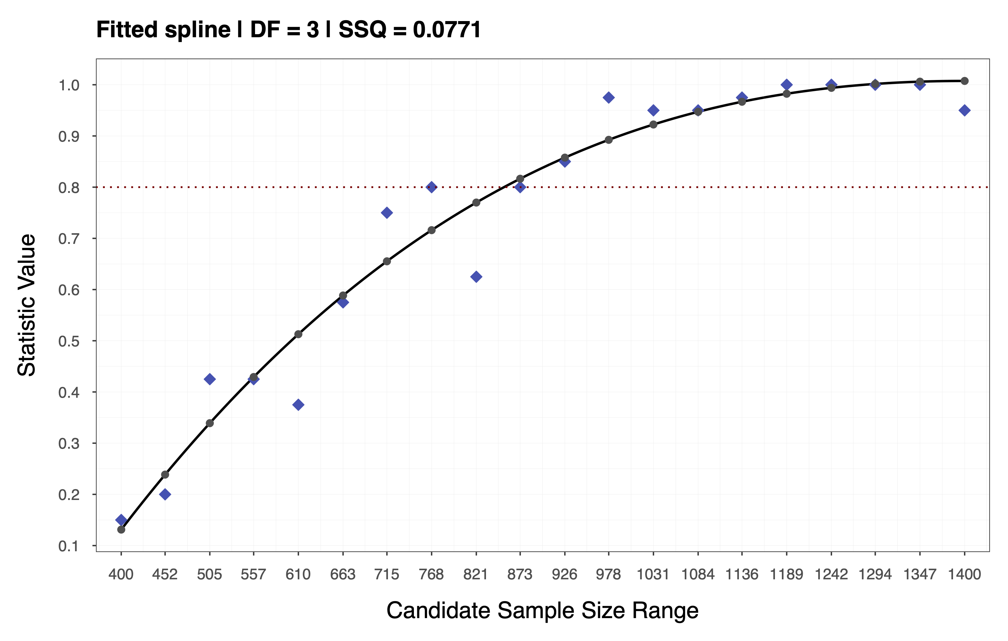
To achieve this, we fit a spline to the statistic values $\mathbf{g}$ obtain in the previous step and use the resulting spline coefficients to interpolate across the entire range ${\mathbb{N}}_s$. Depending on the choice of performance measure and statistic, it may be appropriate to impose monotonicity constraints when fitting the spline. For the example above, we assume a monotone non-decreasing trend and use cubic I-Splines (de Leeuw, 2017; Ramsay, 1988) via the R package splines2 (Wang & Yan, 2021) with the number of inner knots selected based on a cross-validation procedure (e.g., leave-one-out). This assumption implies that the statistic increases as a function of sample size, as depicted in the plot below.

TIP

More information about the second step (i.e., basis functions, spline coefficients, and information about the cross-validation) can be obtained by running plot(results, step = 2), where the results object represents the output provided by the powerly function).

Step 3

The goal of the third step is to quantify the Monte Carlo error around the estimated spline.

To achieve this, we use nonparametric bootstrapping to capture the variability in the replicated performance measures associated with each sample size $s_t\in S$. More specifically, we perform $B$ bootstraps runs, with the index $b(b=1,\dots ,B)$ indicating the current bootstrap run, as follows:

1. Efficiently emulate the MC procedure in Step 1 by sampling with replacement $R$ elements from each vector ${\mathbf{\xi }}_t$ containing the replicated performance measures for the sample size $s_t\in S$.
2. Compute a bootstrapped version of the vector of statistics ${\mathbf{g}}^{(b)}={\left[g\left({\mathbf{\xi }}_1^{(b)}\right),\dots ,g\left({\mathbf{\xi }}_T^{(b)}\right)\right]}^{\top }$, as discussed in Step 1 (i.e., see the animation below).

3. Repeat the spline fitting procedure in Step 2, using as input the the bootstrapped vector of statistics ${\mathbf{g}}^{(b)}$ instead of $\mathbf{g}$. Then, use the resulting bootstrapped spline coefficients to interpolate across the entire range ${\mathbb{N}}_s$.

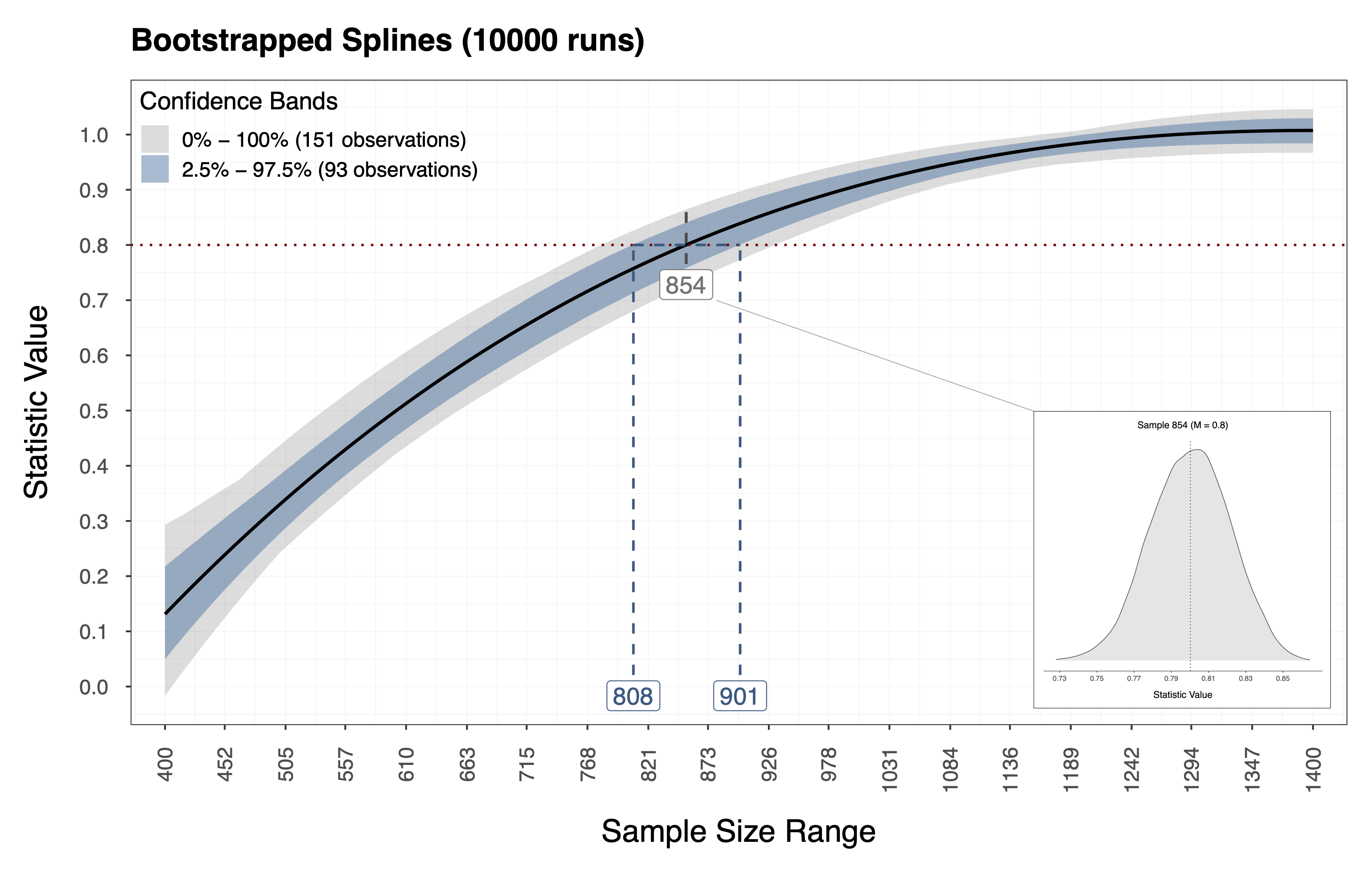
Performing the procedure above gives us a bootstrap distribution of statistic values for each sample size in the candidate range ${\mathbb{N}}_s$. In addition, we obtain this information using relatively few computational resources since we resample the performance measures directly and thus bypass the model estimation and data generation steps. Therefore, using this information we can compute Confidence Intervals (CI) around the observed spline we fit in Step 2. The plot below shows the observed spline (i.e, the thick dark line) and the resulting CI (i.e., the gray and blue bands) for the example above. Furthermore, the distribution depicted below shows the bootstrapped statics associated with a sample size (i.e., $854$ in this case).

Iterations

At this point, we can decide whether subsequent method iterations are needed by zooming in on intersection of the CI and the target value $\tau$ for the statistic (i.e., see the plot below).

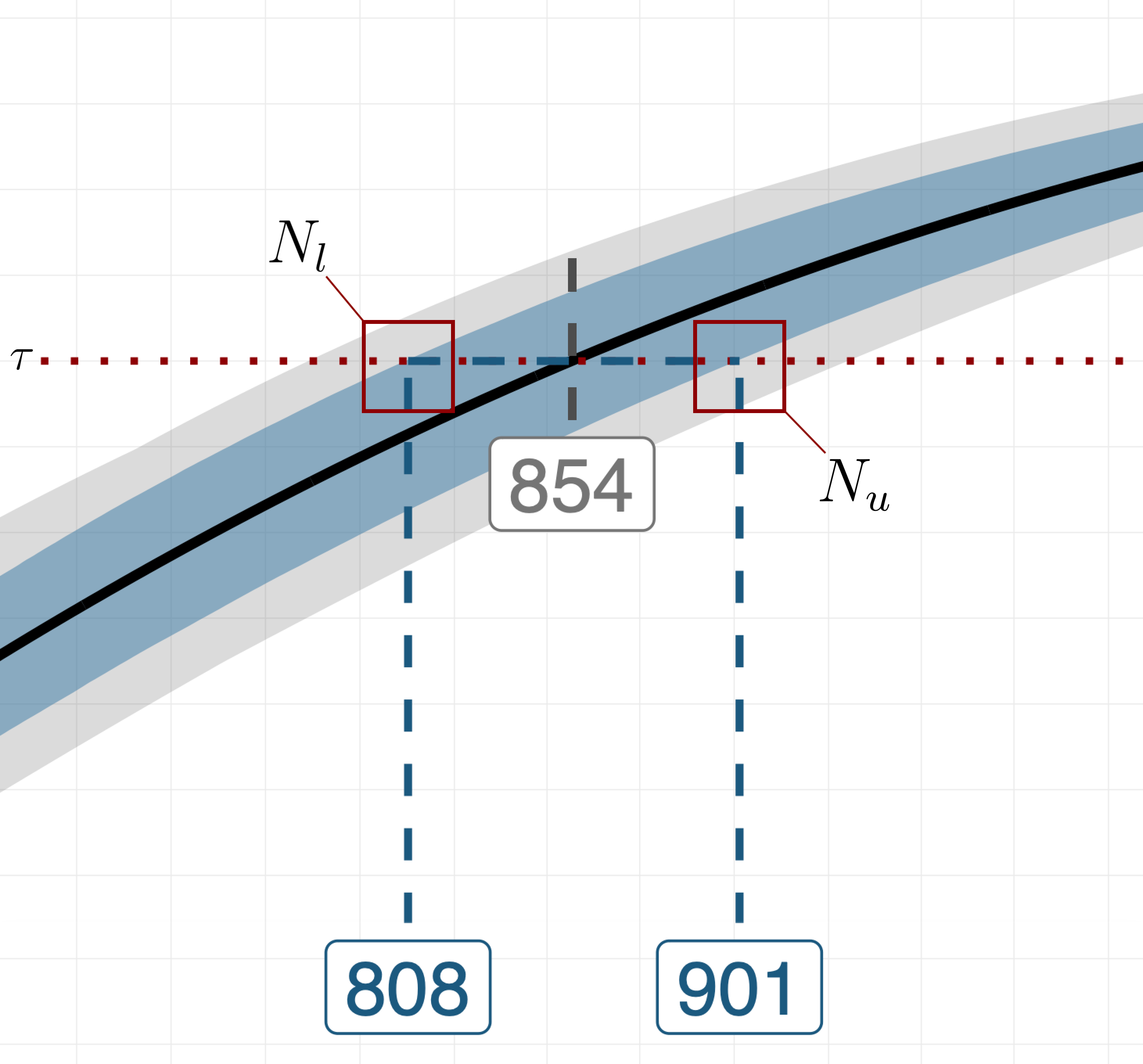
More specifically, we let $N_l$ and $N_u$ be the first sample sizes for which the upper and lower bounds of the $95\%$ CI reach the target value $\tau$. Deciding whether subsequent method iterations are needed boils down to computing the distance between $N_l$ and $N_u$ and comparing it to a scalar $\epsilon$ that indicates the tolerance for the uncertainty around the recommended sample size. If $N_u-N_l\ge \epsilon$, the initial candidate range ${\mathbb{N}}_s$ is updated by setting its lower and upper bounds to $N_l$ and $N_u$, respectively. Then, we repeat the tree steps of method discussed above, this time concentrating the new set of MC replications on the updated and narrowed-down range of sample sizes, i.e., ${\mathbb{N}}_s=[N_l..N_u]$. The algorithm continues to iterate until either $N_u-N_l\ge \epsilon$, or a certain number of iterations has been elapsed.

Implementation

As discussed in the introduction of the Tutorial Section, the main function powerly implements the sample size calculation method described above. When using the powerly function to run a sample size analysis, several arguments can be provided as input. For example, the function signature for consists of the following arguments:

# Arguments supported by `powerly`.
powerly(
  range_lower,
  range_upper,
  samples = 30,
  replications = 30,
  model = "ggm",
  ...,
  model_matrix = NULL,
  measure = "sen",
  statistic = "power",
  measure_value = 0.6,
  statistic_value = 0.8,
  monotone = TRUE,
  increasing = TRUE,
  spline_df = NULL,
  solver_type = "quadprog",
  boots = 10000,
  lower_ci = 0.025,
  upper_ci = 0.975,
  tolerance = 50,
  iterations = 10,
  cores = NULL,
  backend_type = NULL,
  save_memory = FALSE,
  verbose = TRUE
)

WARNING

Please note that the function signature of powerly will change (i.e., be simplified) with the release of the version 2.0.0.

These arguments can be grouped in three categories:

1. Researcher input.
2. Method parameter.
3. Miscellaneous.

The table below provides an overview of the mapping between the notation used in Constantin et al. (2021) and the R function arguments. The order of the rows in the table is indicative of the order in which the arguments appear in the method steps.

Notation	Argument	Category	Description
${\mathbb{N}}_s$	range_lower and range_upper	param	The initial candidate sample size range to search for the optimal sample size.
$T$	samples	param	The number of sample sizes to select from the candidate sample size range.
$R$	replications	param	The number of MC replications to perform for each sample size selected from the candidate range.
$\mathbf{\Theta }$	model_matrix	input	The matrix of true parameter values.
-	model	input	The type or family of true model.
$f\left(\mathbf{\Theta },\hat{\mathbf{\Theta }}\right)$	measure	input	The performance measure.
$\delta$	measure_value	input	The target value for the performance measure.
$g(\mathbf{\xi })$	statistic	input	The statistic (i.e., the definition for power).
$\tau$	measure_value	input	The target value for the statistic.
-	monotone	param	Whether to impose monotonicity constraints on the fitted spline.
-	increasing	param	Whether the spline is assumed to be monotone non-decreasing or increasing.
-	spline_df	param	The degrees of freedom to consider for constructing the basis matrix.
-	solver_type	param	The type of solver for estimating the spline coefficients.
$B$	boots	param	The number of bootstrap runs.
-	lower_ci and upper_ci	param	The lower and upper bounds of the CI around the fitted spline.
$\epsilon$	tolerance	param	The tolerance for the uncertainty around the recommended sample size.
-	iterations	param	The number of method iterations allowed.
-	cores	misc	The number of cores to use for running the algorithm in parallel.
-	backend_type	misc	The type of cluster to create for running the algorithm in parallel.
-	save_memory	misc	Whether to save memory by limiting the amount results stored.
-	verbose	misc	Whether information should be printed while the method is running.

TIP

For more information about the data types and default values for the arguments listed above, consult the Reference Section for the powerly function, or the documentation in R by via ?powerly.

Validation

Aside for the method steps discussed earlier, we can also perform a validation check to determine whether the sample size recommendation consistently recovers the desired value $\delta$ for the performance measure according to the statistic of interest. To achieve this, we repeat the MC procedure described in Step 1, with only one selected sample size, namely, the recommendation provided by the method. This results in a vector of replicated performance measures for which compute the statistic of interest. In order to trust the sample size recommendation, the value of the statistic obtained during the validation procedure should be close to the target value specified by the researcher.

TIP

Check out the Reference Section for the validate function for more details on how validate a sample size recommendation.

References

Constantin, M., Schuurman, N. K., & Vermunt, J. (2021). A General Monte Carlo Method for Sample Size Analysis in the Context of Network Models. https://doi.org/10.31234/osf.io/j5v7u

de Leeuw, J. (2017). Computing and Fitting Monotone Splines. http://dx.doi.org/10.13140/RG.2.2.36758.96327

Knuth, D. E. (1992). Two Notes on Notation. The American Mathematical Monthly, 99(5), 403–422. https://doi.org/10.1080/00029890.1992.11995869

Ramsay, J. O. (1988). Monotone Regression Splines in Action. Statistical Science, 3(4), 425–441. https://doi.org/10.1214/ss/1177012761

Wang, W., & Yan, J. (2021). Shape-restricted regression splines with R package splines2. Journal of Data Science, 19(3), 498–517. https://doi.org/10.6339/21-JDS1020

References

Constantin, M. A., Schuurman, N. K., & Vermunt, J. K. (2023). A General Monte Carlo Method for Sample Size Analysis in the Context of Network Models. Psychological Methods. https://doi.org/10.1037/met0000555